Use of Statistics Glossary Class 10
| What are Subsets | Subsets of Data | Two-way Frequency table |
| Mean | Median | Mean VS Median |
| Median Outliners | Mean Absolute Deviation (MAD) | Standard Deviation (SD) |
Intro to Statistics in Data Science
In previous classes of data sciences you have studies about Arranging and Collecting Data, Data Visualization and Ethics of Data science. Now we’ll cover the how statistical concepts like what are subsets, what is mean, median and relative frequency and how they are used in Data science.
What are Subsets?
Instead of working with the whole data set, we can take a certain part of data for our analysis. This division of small set of data from a large set of data is known as a Subset.
For example, when you visit a restaurants you place your order from the menu. Suppose the menu contains 44 dishes but you only order the ones you want, let’s assume 10. So the 10 dishes that you have ordered is the subset of the whole menu.
The 10 dishes of your order is the relative set of data that is connected to you, and will be your Subset
Subsetting the data is a useful indexing feature for accessing object elements. It can be used for selecting and filtering variables and observations. We subset the data from a data frame to retrieve a part of the data that we need for a specific purpose (in this chase your order). This helps us to observe just the required set of data by filtering out unnecessary content.
Subsets of Data?
Consider a month with 28 days with 1st day as monday and 7th days as sunday so we can picturize something like this,
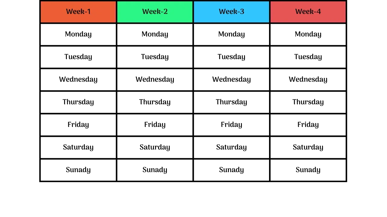
Now let’s understand different ways of subsetting the data.
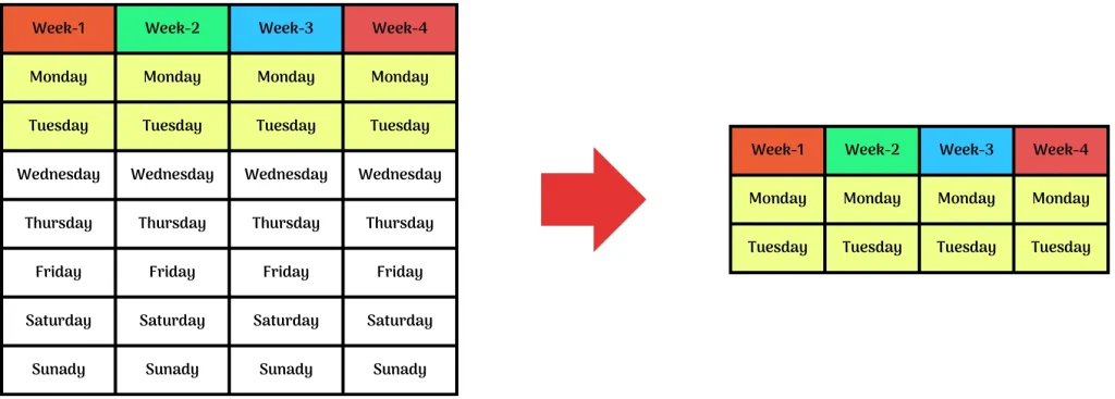
Row-based Subsetting
As the name suggests we take either the top 2 or bottom 2 that is Monday-Tuesday or Saturday-Sunday, this way of selective data is called Row-Based Subsetting.
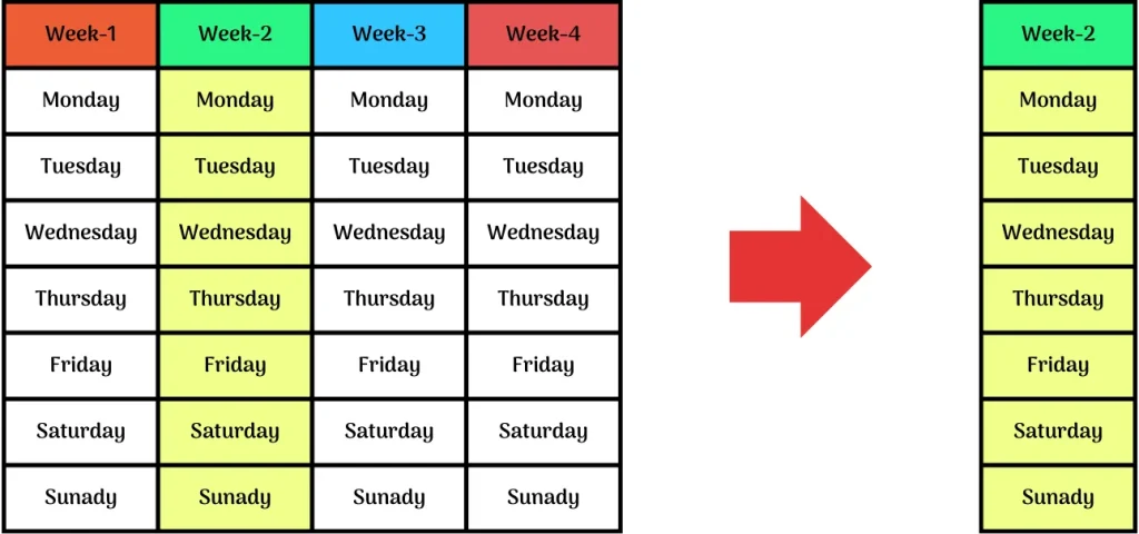
Column-based Subsetting
Same as from the row based subsetting, here we select column that is Week – 1 or Week – 2 from the month, this process of subsetting is known as column-based subsetting.
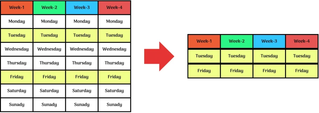
Data-based Subsetting
To subset the data based on specific data we use data-based subsetting. In the above figure, we have selected only those rows which are colored.
Suppose every week on Tuesday and Friday you have Games period in your school, you have based on selective data that’s is your games period sliced your data in a shorter form, this is what we call Data-Based Subsetting.
Two-way Frequency table
A two-way table is a statistical table that demonstrates the observed number or frequency for two variables, the rows indicate one category, and the columns indicate the other category. .
It is simply a table which has two category that defines two different sets of data. One in the form of row and other in column and each value is counted a one value.
Two-way frequency tables show how many data points fit in each category. The row category in this example is “5-10 years”, “10-15 years” and “15-20 years”. The column category is their choice “Like chocolates” or “Do not like chocolates”. Each cell tells us the number (or frequency) of the people.
There is a lot of information that we can get from this small table. For example
1.How many people were questioned ?
Answer
10
2.How many people like chocolates ?
Answer
6
3.In which age group do people like chocolate the most?
Answer
10 – 15
Interpreting two-way tables
The entries in the table are counts. The table has several features:
- Categories are in the left column and top row
- The counts are placed in the center of the table.
- The totals are at the end of each row and column.
- A sum of all counts (a total) is placed at the bottom right
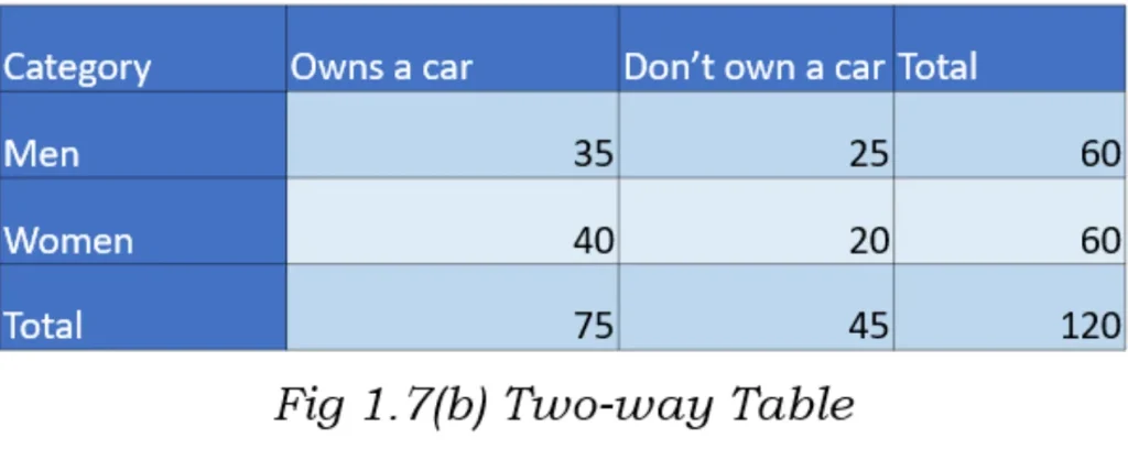
In the above diagram as you can see, the rows of the table tell us whether it’s a Male or a Female and the columns of the table tell us if they own a car or not. Each cell tells us the number (or frequency) of people.
Two-way relative frequency table
Two-way relative frequency table very similar to the two-way frequency type of table. Only difference here is we consider percentage instead of numbers.
Two-way relative frequency tables represent what is the percentage of data points that fit in each category.
We can take help of row relative frequencies or column relative frequencies; it totally depends on the context of the problem. Let us consider the below two-way table recording preferences of boys and girls with regards to indoor and outdoor sports.
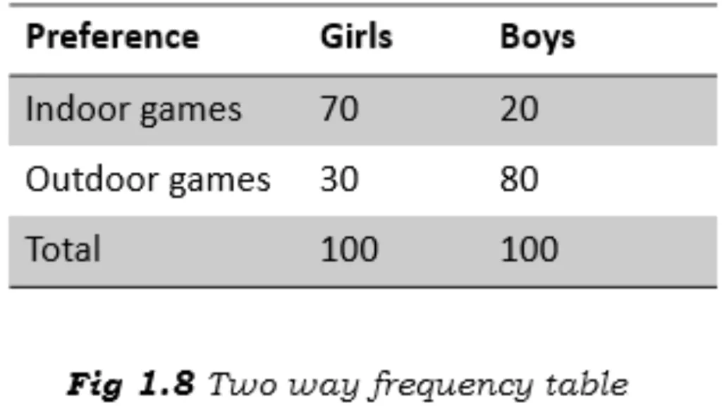
To convert this into a relative two-way frequency table we will convert individual cells into percentages.
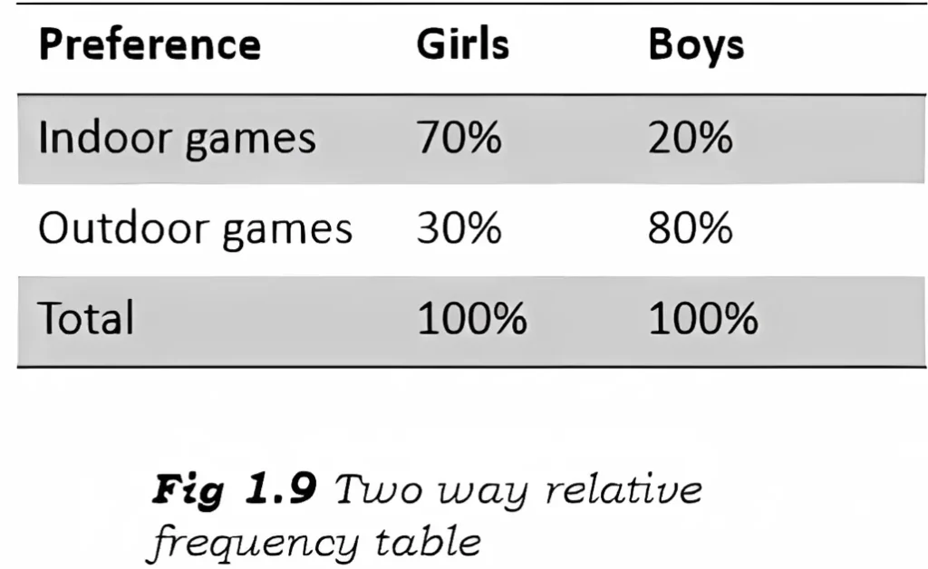
Two-way relative frequency tables are helpful when there are different sample sizes in a dataset. Percentages makes it easier to compare the preferences.
Meaning of mean
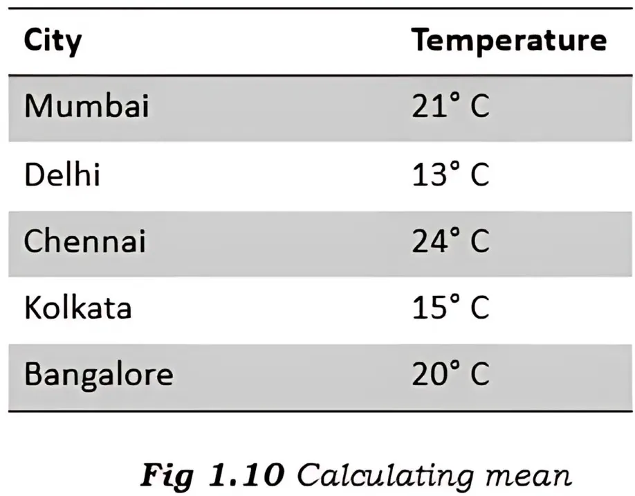
Mean is a measure of central tendency. In data science, Mean, also termed as the simple average, is an average value of a data set. Basically, mean is a value in the data set around which entire data is spread out.
While mean is calculated, all values used in calculating the average are weighted equally.
The mean of a data set is calculated by adding up all the values in the data set and later dividing them by the number of values present in the data frame.
Example
- Consider that we have a set of 11 numbers 10 to 20 in a data set.
- Array = {10, 11, 12, 13, 14, 15, 16, 17, 18, 19, 20}
- So mean is calculated by adding up 10 numbers in the data set.
- Sum of all the numbers = 165
- Mean = 165/10 = 16.5
Median
Two-way relative frequency tables represent what is the percentage of data points that fit in each category.
To calculate median, we must order our data set in ascending or descending order. If the data set is sorted from smallest value to biggest value, the exact middle value of the set is the Median.
Example
ODD no of elements
- Array = [12, 34, 56, 89, 32]
- Sorted array = [12, 32, 34, 56, 89]
- The value at 3rd position is the middle point of the sorted list. So, 34 is our median for the array.
[12, 32, 34, 56, 89] hence 34 is the median
NOTE: 34 is selected as the median after we have sorted the Array
EVEN no of elements
- Array = [12, 34, 56, 89, 32, 48]
- Sorted array = [12, 32, 34, 48, 56, 89]
we need to calculate the average of these two numbers to get the median - Hence median is 34 + 48 = 72
72/2 = 36
Median Outliners
Let’s understand this with an example:
Assume that Lalit gets his blood pressure checked every week. But due some error in the device, the recording for one week was too high.
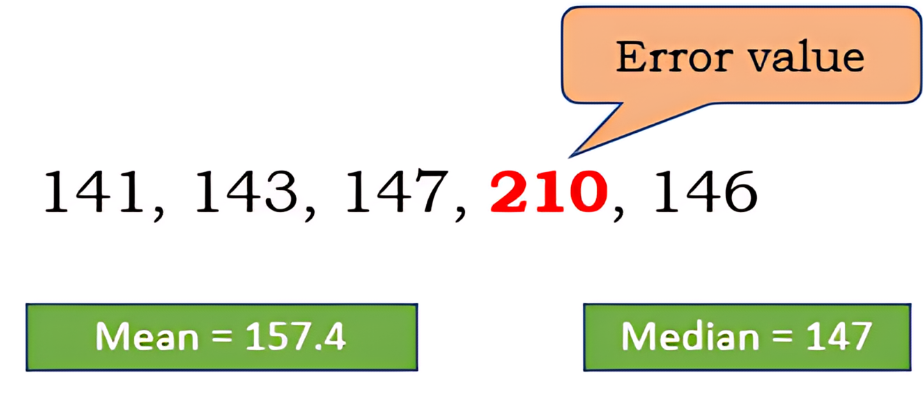
Here the outliner value is 210
So, for the above scenario we see the mean value deviates greatly from the regular blood pressure values due to a device error. Whereas the median value still accurately represents the central point of the data set. So under circumstances where there are outliers in the data set, median is a more effective measure of central tendency.
Mean VS Median
Mean
- Its is the average value of the whole list or Array
- Even no of elements: add all the elements and divide the sum with the no of elements.
- Odd no of elements: add all the elements and divide the sum with the no of elements.
Median
- Median is the middle element of the list irrespective.
- Even no of elements: add the center elements after sorting the list and divide by 2
- Odd no of elements: Middle element of the sorted list.
- Median is a more accurate form of central tendency specially in scenarios where there are some irregular values also known as Outliers
Mean Absolute Deviation (MAD)
The average of how far away all values in a data set are from the mean.
Example
Consider the data set – [12, 16, 10, 18, 11, 19]
Step 1:
Calculate the mean
Mean = (12 + 16 + 10 + 18 + 11 + 19) /6 = 86/6 = 14.333333 = 14 (rounded off)
Step 2:
Calculate the distance of each data point from the mean. We need to find the absolute value.
For example if the distance is -2, then we ignore the negative sign.
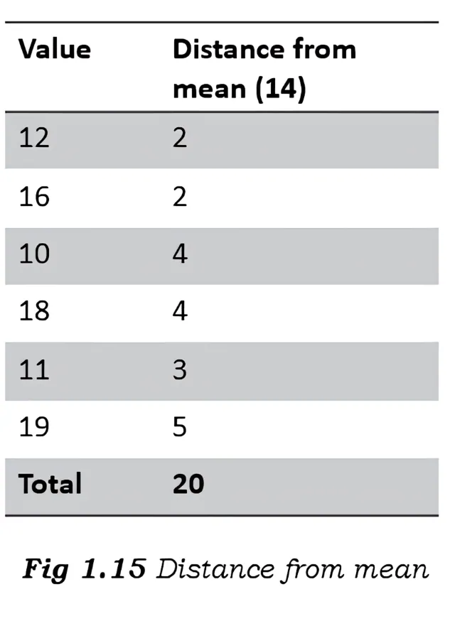
Step 3:
Calculate the mean of the distances.
Mean of distances = (2 + 2 + 4 + 4 + 3 + 5) / 6 = 3.33
So 3.33 is our mean absolute deviation, and the mean is 14.
The value of Mean absolute deviation gives a very good understanding of the variability of the data set.
Standard Deviation (SD)
standard deviation represents how much the data is spread out around the mean or an average.
To find standard deviation:
- Calculate the mean by adding up all the data pieces and dividing it by the number of pieces of the data.
- Subtract mean fromevery value
- Square each of the differences
- Find the average of squared numbers calculated in point number 3 to find the variance.
- Lastly, find the square root of variance. That is the standard deviation.
Example
Values; [1, 2, 3, 5, 8]
- Calculate the mean
1+2+3+5+8 = 19
19/5 = 3.8 (mean) - Subtract mean from every value
1- 3.8= -2.8
2- 3.8= -1.8
3- 3.8= -0.8
5- 3.8= 1.2
8- 3.8= 4.2 - Square each difference
(-2.8)*(-2.8) = 7.84
(-1.8)*(-1.8) = 3.24
(-0.8)*(-0.8) = 0.64
(1.2)*1.2) = 1.44
(4.2)*(4.2) = 17.64 - Calculate the average of the squared numbers to get the variance
7.84+3.24+0.64+1.44+17.64 = 30.8
30.8/5 = 6.16 (Variance) - Find the square root of the variance
The square root of 6.16 = 2.48
Thus, the Standard deviation of values 1,2,3,5 and 8 is 2.48.
